
LLMs from the Inside 2: Word Embedding
Hi guys! John the Quant here. In this series of articles, we are going to explore each piece of the architecture that makes models like GPT, Llama, and Claude possible. All of the big, generative Large Language Models follow the same basic architecture. It looks like this:

All of the big LLMs follow this general structure.
As we talk about each piece, we are going to explore different implementation options, which famous models use which option, and why the designers made that choice.
Let’s get started.
Where We Are
In Part 1, we explored tokenizers like Byte-Pair Encoding and WordPiece. The text goes into the tokenizer and comes out as a sequence of integers like in the example below.

A tokenizer takes in text and returns a meaningful sequence of integers.
Large Language Models can only really “understand” numbers, so we’ve turned the input text into something the model can work with.
Semantic Arithmetic
Integers don’t carry much information by themselves, and a single number certainly can’t convey all the information we get from a word. Here is a classic example.
If I tell you a person is a King, what else do you know? You know the person is royal, and is male, that they lead a country and that their family is also royalty. That’s a lot of information from just a single word. We’re going to need more than a single number to convey that much information. This implies that words are multi-dimensional.
Now, what’s the difference between a King and a Queen? Most of the information in the previous paragraph is true of either a king or a queen. The only difference is gender: King implies Male and Queen implies Female. We have stumbled upon a kind of “semantic arithmetic”.

We can add and subtract concepts from words to get new words!
On the subject of monarchs, who do you think was a better ruler, Alexander the Great of Macedonia (336–323 B.C.E.) or Ashoka the Great of Magadha (304–232 B.C.E)? Read their Wikipedia pages before you answer. Certainly, they were both great leaders of history. But we’ve just opened up another question for computational linguistics: How do we get from “good” to “better”? And what about “best”? These words carry magnitude! Something that is 1.5 times as “good” as another thing is “better”, right? And something that is the “best” is “better” than the others! We can interpret “better” as “good” with a multiplier greater than one and “best” as “good” with the highest multiplier. This means semantic arithmetic must include multiplication.
Words have addition, subtraction, multiplication, and division. Complete semantic arithmetic.
We’ve established that words are multi-dimensional and that they have direction, magnitude, and the big four arithmetic functions. Vectors are multi-dimensional, they have direction and magnitude, the four big arithmetic functions are defined on vectors, and (importantly!!) vector space is closed under addition, subtraction, multiplication, and division. This means that if we add, subtract, multiply, or divide any two vectors, we get another vector. That’s important! If we put vectors in and got something other than a vector out, we couldn’t use vectors for word meaning! We put words in and we need to get words out.
Thus, we are going to use a vector as a mathematical approximation of a word’s meaning. That’s the idea behind Word Embedding, the next part of our Language Model.
Word Embedding
Words have two different types of meaning. There is a constant meaning and a contextual meaning. When you look up a word in the dictionary, you get the constant meaning; the meaning of the word in general, regardless of how the word is used. But we also know that the meaning of a word depends on how it is being used; that’s the contextual meaning. In a Large Language Model, Word Embedding captures the constant meaning and Positional Encoding — the focus of the next article in the series — provides the contextual meaning.
Think of Word Embedding like looking up the word in a dictionary. In a dictionary, you find the definition that corresponds to your word and get a sequence (of words) that defines the meaning of your word. In a Word Embedding, you find the vector that goes along with your token and get a vector (of numbers) that defines the meaning of your token.
That’s all a Word Embedding layer is: A big lookup table.

An embedding layer is basically a lookup table.
Training
Neural Networks are trained with backpropagation, and we also want the Word Embedding to be trainable via backpropagation. A lookup table cannot be trained, but it is mathematically identical to multiplying a one-hot encoded vector with the matrix of embedding vectors. See the image below.

A lookup table is the same as multiplying a matrix by a one-hot vector! And we can train this using backpropagation.
A lookup table is more computationally efficient than matrix multiplication, so we will treat the Word Embedding layer as a lookup table as often as possible. But matrix multiplication is differentiable, so we will treat it as a Linear layer with no bias for training.
Embedding layers can be trained using self-supervised learning. Simply get sequences of tokenized text and predict the next token. While pretrained embedding layers exist, most LLMs train their own embedding layers along with the rest of the model for maximum flexibility.
Alternative Embedding Algorithms
While all the major generative LLMs use the simple implementation described above, scientists have been developing numerical representations of word meaning for decades. The following three embedding algorithms were major breakthroughs in semantic representation and are still used today.
Word2Vec
This embedding algorithm was developed at Google and released in 2013. It was a huge jump forward in natural language understanding for machines. The algorithm used in LLMs — described in the previous section — is a sub-algorithm of Word2Vec.
Word2Vec is always a two-layer neural network. The first layer takes in the tokens and maps them to the embedding. The second layer takes the embeddings and maps them to the output via Softmax function. The second layer is used for training and then discarded.
Continuous Bag of Words
In this mode, we train the model to fill in the blank. One token of the input sequence is the target, and the rest of the words are used to predict the missing word. This trains the embedding vectors for each of the input words simultaneously, but it struggles to map rare words.
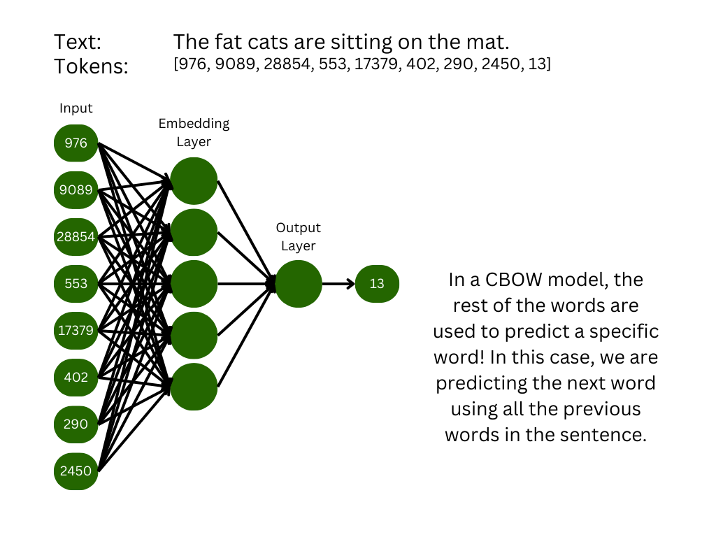
In continuous bag of words, you set aside one word and use the rest of the text to predict that word.
Skip-Gram
This mode is the opposite of the CBOW: All words but one are the targets, and the single input word is used to predict all of the others. This method trains much slower but is more effective for rare words as the single input word receives the full gradient.

In a skip-gram model, you take one word from the text and learn to predict what other words occur nearby.
GloVe
This algorithm was developed at Stanford as a competitor to Word2Vec and was released in 2014. Instead of using a neural network to find word embeddings, GloVe uses matrix factorization. You start off by defining a context-window. This is a sliding window in which words are related. See the image below.

The context window slides over the token sequence.
Now, you slide the context window over the entire corpus and count how many times each pair of tokens occurs together. This creates the word-context matrix.

This co-occurrence matrix is really simple because the corpus is one sentence with no repeated words.
The last step of GloVe is to factor the word-context matrix, yielding two matrices: The Word Embedding matrix and a context matrix.

We factor the co-occurrence matrix to get the word embedding matrix.
Because these embedding vectors are based on word co-occurrence, they appear to be more interpretable and meaningful than neural-network vectors like in Word2Vec. I have some concerns about that interpretation, but it seems to be a common thought.
fastText
This algorithm was developed by Facebook AI Research and released in 2016. But let’s not fool ourselves: It is basically the same as Word2Vec. Tokens are fed into a linear neural network layer in a CBOW fashion and used to predict the next word. The big upgrade from the original Word2Vec is the use of hierarchical softmax for the output, which reduces the asymptotic complexity from O(embedding dimension * vocab size) to O(embedding dimension * log_2(vocab size)). That’s a huge improvement in computational efficiency.
Conclusion
In this article, we explored the reasoning behind Word Embeddings and how they help Large Language Models generate human-like text. All of the big LLMs use embedding layers, which are lookup tables but are treated like linear layers during training. We then discussed three popular embedding algorithms:
Word2Vec — Training a two-layer neural network to either predict the next word or fill-in-the-blank, then using the output from the hidden layer as the embedding.
GloVe — Using matrix factorization on a word co-occurrence matrix to separate the word meaning from the contextual meaning.
fastText — Applying the same method as Word2Vec to subword tokens and using hierarchical softmax to make it more computationally efficient.
Theoretically, any embedding algorithm should work in an LLM. You could even use a pre-trained embedding! However, embeddings are tied to tokenizers, so if you use a pre-trained embedding you must use the same tokenizer used for training it. The way the big LLMs handle embedding layers allows you to train the embedding specifically to work best with your data and the rest of your model. Still, you might consider using a pre-trained embedding if you want to use a smaller training corpus.